Comparison splinebox and scipy: edge fitting

This example compares splinebox and scipy when trying to fit a spline to an end of an image.

# sphinx_gallery_thumbnail_number = 2

import cycler
import matplotlib as mpl
import matplotlib.pyplot as plt
import numpy as np
import scipy
import scipy.optimize
import skimage
import splinebox

First, we will set some defaults to style our plot. You can ingnore this section if you don’t care about the style of the plots.

mpl.rcParams["image.cmap"] = "gray"
mpl.rcParams["lines.linewidth"] = 2
mpl.rcParams["axes.prop_cycle"] = cycler.cycler(color=("r",))

In this example, we will use a crop of the scikit-image’s text example image.

img = skimage.data.text()
img = img[45:78, 300:430]
plt.imshow(img)
plt.show()

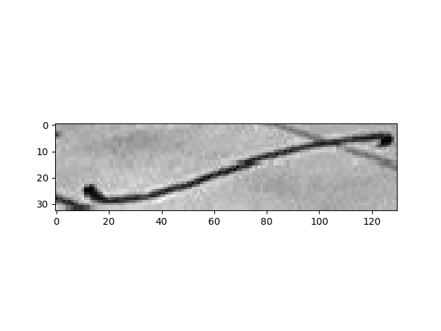
Our goal is to fit a spline to the integral sign on the page. We won’t cover how to automatically find a good initial guess but instead just select five pixels that are more or less equally spaced along the integral as the initial not of our spline.

initial_knots = np.array([[24, 12], [23, 47], [16, 72], [8, 97], [8, 124]])

In order to evaluate how well our spline fits the line, we will have to interpolate the pixel values at non-integer position. Since the line is black on a white background, our goal is to move the spline in a way that minimises the average pixel value under it. This is commonly refered to as the image energy.

interpolator = scipy.interpolate.RectBivariateSpline(np.arange(img.shape[0]), np.arange(img.shape[1]), img, s=1)

We will start by constructing an initial spline using splinebox.

M = len(initial_knots)
basis_function = splinebox.B3()
spline = splinebox.Spline(M, basis_function, closed=False)
spline.knots = initial_knots

Let’s define the parameter values at which we want to sample the spline. Here, we chose to sample 50 points inbetween two knots.

t = np.linspace(0, M - 1, M * 50)

In order to compar the fitted spline to the intial one, we save it’s positions and knots for plotting later on.

initial_vals = spline.eval(t)
initial_knots = spline.knots

Before we can start fitting the spline, we have to define the loss function. In this example our loss function consists of two parts, the image energy, discussed above and an internal energy. Here, we choose to use the curvilinear reparametrization energy as our internal energy. It promotes equidistant spacing of the knots in terms of arc length. In practice, this avoids sharp bends and stops the spline from looping/folding back on itself. Without it, the image energy would reward the spline for visiting the darkest pixels multiple times. The parameter alpha can be used balance the contribution of the image and internal energies.

def loss_function_splinebox(control_points, alpha):
    spline.control_points = control_points.reshape((-1, 2))
    coordinates = spline.eval(t)
    image_energy = np.mean(interpolator(coordinates[:, 0], coordinates[:, 1], grid=False))
    internal_energy = spline.curvilinear_reparametrization_energy()
    return image_energy + alpha * internal_energy

For the fitting procedure we can simply use scipy. The value for alpha was empirically set to 500.

initial_control_points = spline.control_points
scipy.optimize.minimize(loss_function_splinebox, initial_control_points.flatten(), args=(500,))

 message: Optimization terminated successfully.
 success: True
  status: 0
     fun: 36.84064228311857
       x: [-1.546e+01  1.866e+01 ...  2.018e+01  5.141e+01]
     nit: 119
     jac: [ 9.537e-07  4.768e-07 ...  0.000e+00  4.768e-07]
hess_inv: [[ 1.282e+02 -6.134e+01 ...  1.102e+01  1.306e+01]
           [-6.134e+01  3.748e+02 ... -2.810e+01  8.961e+01]
           ...
           [ 1.102e+01 -2.810e+01 ...  1.693e+02 -9.179e+01]
           [ 1.306e+01  8.961e+01 ... -9.179e+01  3.397e+02]]
    nfev: 2055
    njev: 137

Let’s plot the results.

fitted_vals = spline.eval(t)
fitted_knots = spline.knots

fix, axes = plt.subplots(2, 1, sharex=True, sharey=True)
axes[0].imshow(img)
axes[0].plot(initial_vals[:, 1], initial_vals[:, 0], label="initial spline")
axes[0].scatter(initial_knots[:, 1], initial_knots[:, 0], label="initial knots")
axes[0].legend()
axes[1].imshow(img)
axes[1].plot(fitted_vals[:, 1], fitted_vals[:, 0], label="fitted spline")
axes[1].scatter(fitted_knots[:, 1], fitted_knots[:, 0], label="fitted knots")
axes[1].legend()
plt.suptitle("SplineBox")
plt.tight_layout()
plt.show()

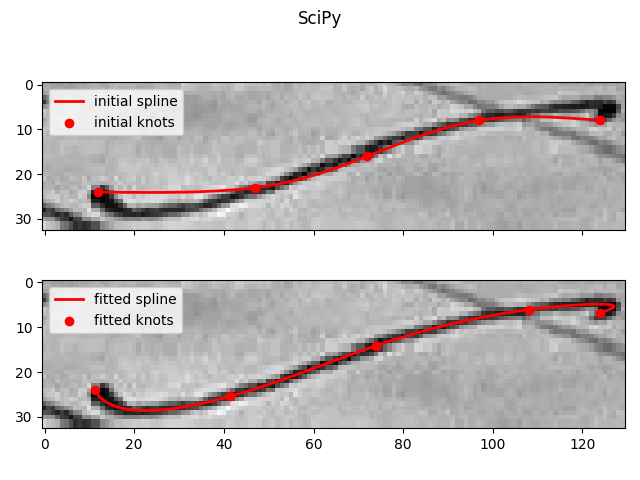
Next, we will try to acchive the same fit using scipy. As before, we begin by construcing an initial spline using the initial knots. NOTE: you have to set bc_type in order to get a spline with the desired number of knots.

k = 3
t_knots = np.arange(M)
spline = scipy.interpolate.make_interp_spline(t_knots, initial_knots, k=3, bc_type="natural")

initial_vals = spline(t)
initial_knots = spline(spline.t)[k:-k]

Since scipy does not provide a function to compute the curvilinear reparametrization energy, we have to do it ourselfs.

def loss_function_scipy(control_points, alpha):
    spline.c = control_points.reshape((-1, 2))
    coordinates = spline(t)
    image_energy = np.mean(interpolator(coordinates[:, 0], coordinates[:, 1], grid=False))
    derivative = spline.derivative()
    integral = scipy.integrate.quad(lambda t: np.linalg.norm(derivative(t)), 0, M - 1)
    length = integral[0]
    c = (length / M) ** 2
    integral = scipy.integrate.quad(lambda t: (np.linalg.norm(derivative(t)) ** 2 - c) ** 2, 0, M - 1)
    internal_energy = integral[0] / length**4
    return image_energy + alpha * internal_energy


initial_control_points = spline.c
scipy.optimize.minimize(loss_function_scipy, initial_control_points.flatten(), args=(500,))

 message: Optimization terminated successfully.
 success: True
  status: 0
     fun: 36.84064228312302
       x: [ 2.409e+01  1.117e+01 ...  6.737e+00  1.239e+02]
     nit: 68
     jac: [ 1.431e-06  0.000e+00 ...  1.907e-06  2.861e-06]
hess_inv: [[ 9.638e-01  1.367e-01 ...  5.749e-02 -3.243e-03]
           [ 1.367e-01  9.017e-01 ... -5.137e-03 -1.333e-02]
           ...
           [ 5.749e-02 -5.137e-03 ...  1.569e+00 -4.038e-01]
           [-3.243e-03 -1.333e-02 ... -4.038e-01  1.240e+00]]
    nfev: 1215
    njev: 81

Let’s take a look at the results.

fitted_vals = spline(t)
fitted_knots = spline(spline.t[k:-k])

fix, axes = plt.subplots(2, 1, sharex=True, sharey=True)
axes[0].imshow(img, cmap="gray")
axes[0].plot(initial_vals[:, 1], initial_vals[:, 0], label="initial spline")
axes[0].scatter(initial_knots[:, 1], initial_knots[:, 0], label="initial knots")
axes[0].legend()
axes[1].imshow(img, cmap="gray")
axes[1].plot(fitted_vals[:, 1], fitted_vals[:, 0], label="fitted spline")
axes[1].scatter(fitted_knots[:, 1], fitted_knots[:, 0], label="fitted knots")
axes[1].legend()
plt.suptitle("SciPy")
plt.tight_layout()
plt.show()