Note
Go to the end to download the full example code.
Comparison of splinebox and scipy: Edge Fitting#
This example compares the performance of splinebox and scipy when fitting a spline to an image feature, in this case, an integral symbol in a cropped section of an image.
import matplotlib as mpl
import matplotlib.pyplot as plt
import numpy as np
import scipy
import scipy.optimize
import skimage
import splinebox
Plot Styling#
To ensure consistent plot aesthetics, let’s set some default parameters for Matplotlib. This section can be ignored if you do not need custom plot styling.
mpl.rcParams["image.cmap"] = "gray"
mpl.rcParams["lines.linewidth"] = 2
# mpl.rcParams["axes.prop_cycle"] = cycler.cycler(color=("r",))
scipy_blue = "#0053a6"
Load and Display the Image#
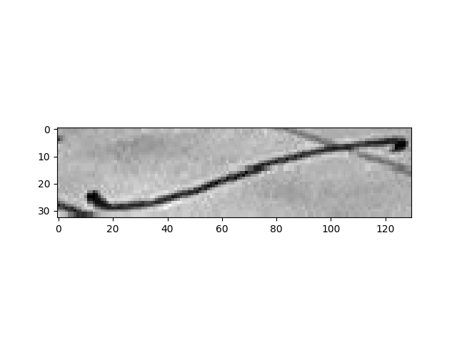
We use a cropped version of the ‘text’ example image from skimage. This section crops image to the portion containing the integral symbol.
img = skimage.data.text()
img = img[45:78, 300:430]
plt.imshow(img)
plt.show()
In order to evaluate how well our spline fits the line, we will have to interpolate the pixel values at non-integer position. Since the line is black on a white background, our goal is to move the spline in a way that minimises the average pixel value under it. This is commonly refered to as the image energy. To be able to quickly interpolate the pixel values, we fit a bivariate spline to the pixel values. The interpolator object is callable and can be querried for pixel coordinates.
interpolator = scipy.interpolate.RectBivariateSpline(np.arange(img.shape[0]), np.arange(img.shape[1]), img, s=1)
Define Initial Knots#
We’ll fit the spline to the integral symbol. Rather than finding initial points automatically, we’ll manually select five points roughly spaced along the integral symbol.
initial_knots = np.array([[24, 12], [23, 47], [16, 72], [8, 97], [8, 124]])
Create a Spline Using splinebox#
We first use splinebox to create a spline from the selected knots.
M = len(initial_knots)
basis_function = splinebox.B3()
spline = splinebox.Spline(M, basis_function, closed=False)
spline.knots = initial_knots
Let’s define the parameter values at which we want to sample the spline. Here, we chose to sample 50 points inbetween knots.
t = np.linspace(0, M - 1, M * 50)
In order to compar the fitted spline to the intial one, we save it’s positions and knots for plotting later on.
initial_vals = spline.eval(t)
initial_knots = spline.knots
Define the Loss Function for splinebox#
Our loss function combines the image energy (to minimize pixel values along the spline) and an internal energy term that ensures smooth, equidistant knots to avoid sharp turns or loops.
Here, we use the curvilinear reparametrization energy as our internal energy.
It promotes equidistant spacing of the knots in terms of arc length.
In practice, this avoids sharp bends and stops the spline from looping/folding back on itself.
Without it, the image energy would reward the spline for visiting the darkest pixels
multiple times.
The parameter alpha can be used balance the contribution of the image and internal energies.
def loss_function_splinebox(control_points, alpha):
    spline.control_points = control_points.reshape((-1, 2))
    coordinates = spline.eval(t)
    image_energy = np.mean(interpolator(coordinates[:, 0], coordinates[:, 1], grid=False))
    internal_energy = spline.curvilinear_reparametrization_energy()
    return image_energy + alpha * internal_energy
Fit the Spline (splinebox)#
We use scipy.optimize.minimize to find the best-fitting spline by minimizing the total energy.
The parameter alpha controls the balance between image energy and internal energy (here emperically set to 500).
initial_control_points = spline.control_points
scipy.optimize.minimize(loss_function_splinebox, initial_control_points.flatten(), args=(500,))
 message: Optimization terminated successfully.
 success: True
  status: 0
     fun: 36.84064228311857
       x: [-1.546e+01  1.866e+01 ...  2.018e+01  5.141e+01]
     nit: 119
     jac: [ 9.537e-07  4.768e-07 ...  0.000e+00  4.768e-07]
hess_inv: [[ 1.282e+02 -6.134e+01 ...  1.102e+01  1.306e+01]
           [-6.134e+01  3.748e+02 ... -2.810e+01  8.961e+01]
           ...
           [ 1.102e+01 -2.810e+01 ...  1.693e+02 -9.179e+01]
           [ 1.306e+01  8.961e+01 ... -9.179e+01  3.397e+02]]
    nfev: 2055
    njev: 137
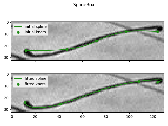
Plot the Results (splinebox)#
Finally, we plot the initial and fitted splines for comparison.
fitted_vals = spline.eval(t)
fitted_knots = spline.knots

fix, axes = plt.subplots(2, 1, sharex=True, sharey=True)
axes[0].imshow(img)
axes[0].plot(initial_vals[:, 1], initial_vals[:, 0], label="initial spline")
axes[0].scatter(initial_knots[:, 1], initial_knots[:, 0], label="initial knots")
axes[0].legend()
axes[1].imshow(img)
axes[1].plot(fitted_vals[:, 1], fitted_vals[:, 0], label="fitted spline")
axes[1].scatter(fitted_knots[:, 1], fitted_knots[:, 0], label="fitted knots")
axes[1].legend()
plt.suptitle("SplineBox")
plt.tight_layout()
plt.show()
Create a Spline Using scipy#
Next, we attempt to achieve the same fit using scipy.
We construct an initial spline with scipy.interpolate.make_interp_spline using the same knots.
NOTE: you have to set bc_type in order to get a spline with the desired
number of knots.
# Spline order
k = 3
# The parameter value for the knots
t_knots = np.arange(M)
spline = scipy.interpolate.make_interp_spline(t_knots, initial_knots, k=3, bc_type="natural")

# Save initial values for comparison
initial_vals = spline(t)
initial_knots = spline(spline.t)[k:-k]
Define the Loss Function for scipy#
Since scipy does not have a built-in curvilinear reparametrization energy, we calculate it manually.
def loss_function_scipy(control_points, alpha):
    spline.c = control_points.reshape((-1, 2))
    coordinates = spline(t)
    image_energy = np.mean(interpolator(coordinates[:, 0], coordinates[:, 1], grid=False))

    # Compute internal energy (curvilinear reparametrization)
    derivative = spline.derivative()
    integral = scipy.integrate.quad(lambda t: np.linalg.norm(derivative(t)), 0, M - 1)
    length = integral[0]
    c = (length / M) ** 2
    integral = scipy.integrate.quad(lambda t: (np.linalg.norm(derivative(t)) ** 2 - c) ** 2, 0, M - 1)
    internal_energy = integral[0] / length**4

    return image_energy + alpha * internal_energy
Fit the Spline (scipy)#
initial_control_points = spline.c
scipy.optimize.minimize(loss_function_scipy, initial_control_points.flatten(), args=(500,))
 message: Optimization terminated successfully.
 success: True
  status: 0
     fun: 36.84064228312302
       x: [ 2.409e+01  1.117e+01 ...  6.737e+00  1.239e+02]
     nit: 68
     jac: [ 1.431e-06  0.000e+00 ...  1.907e-06  2.861e-06]
hess_inv: [[ 9.638e-01  1.367e-01 ...  5.749e-02 -3.243e-03]
           [ 1.367e-01  9.017e-01 ... -5.137e-03 -1.333e-02]
           ...
           [ 5.749e-02 -5.137e-03 ...  1.569e+00 -4.038e-01]
           [-3.243e-03 -1.333e-02 ... -4.038e-01  1.240e+00]]
    nfev: 1215
    njev: 81
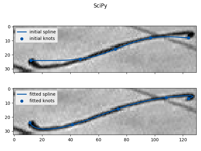
Plot the Results (scipy)#
Finally, we plot the initial and fitted splines for the scipy result.
fitted_vals = spline(t)
fitted_knots = spline(spline.t[k:-k])

fix, axes = plt.subplots(2, 1, sharex=True, sharey=True)
axes[0].imshow(img, cmap="gray")
axes[0].plot(initial_vals[:, 1], initial_vals[:, 0], label="initial spline", color=scipy_blue)
axes[0].scatter(initial_knots[:, 1], initial_knots[:, 0], label="initial knots", color=scipy_blue)
axes[0].legend()
axes[1].imshow(img, cmap="gray")
axes[1].plot(fitted_vals[:, 1], fitted_vals[:, 0], label="fitted spline", color=scipy_blue)
axes[1].scatter(fitted_knots[:, 1], fitted_knots[:, 0], label="fitted knots", color=scipy_blue)
axes[1].legend()
plt.suptitle("SciPy")
plt.tight_layout()
plt.show()
Total running time of the script: (0 minutes 37.667 seconds)