Comparison splinebox and scipy: contour approximation

This example compares splinebox and scipy when trying to approximate a contour/shape with a closed spline with a fixe number of control points.

import matplotlib.pyplot as plt
import numpy as np
import scipy
import skimage
import splinebox

scipy_blue = "#0053a6"

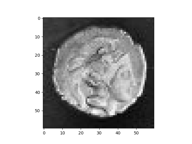
Let’s load the astronaut example image from skimage and crop out a single coins using slicing.

img = skimage.data.coins()[90:150, 240:300]
plt.imshow(img, cmap="gray")
plt.show()

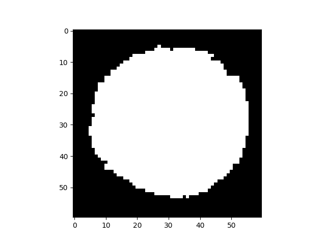
Next, we will segment the coin using Otsu’s method and fix some holes in the mask.

thresh = skimage.filters.threshold_otsu(img)
mask = img > thresh
mask = skimage.morphology.remove_small_holes(mask)
plt.imshow(mask, cmap="gray")
plt.show()

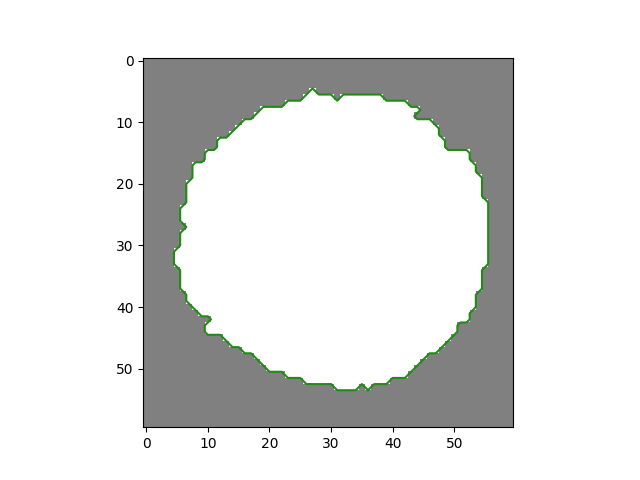
We can find the contour of the coin using find contours. The return value is a list of contours. Since our binary image only has one contour we select the first element of the list.

contours = skimage.measure.find_contours(mask)
contour = contours[0]
plt.imshow(mask, cmap="gray", alpha=0.5)
plt.plot(contour[:, 1], contour[:, 0])
plt.show()

For closed contours, the last point is identical to the first one, so we will chop it off.

contour = contour[:-1]

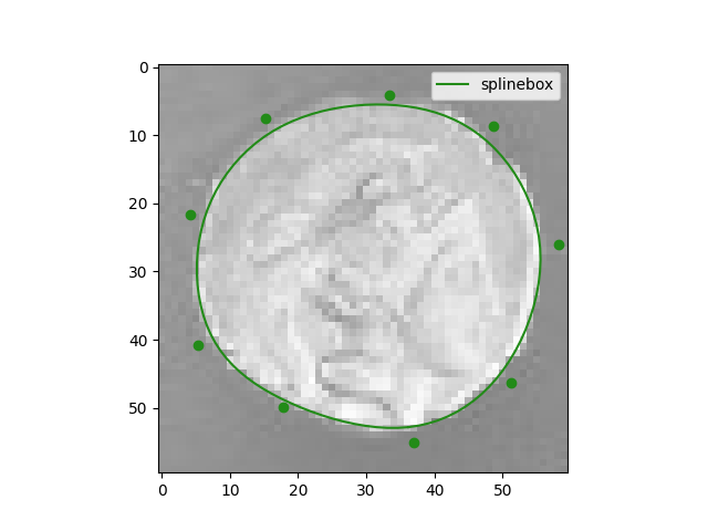
Our goal is to fit a cubic B-spline with M control points to the contour. We will first use splinbox to acchive this and then use scipy.

M = 9

spline = splinebox.Spline(M=M, basis_function=splinebox.B3(), closed=True)
spline.fit(contour)

ts = np.linspace(0, M, 100)
splinebox_vals = spline(ts)
splinebox_control_points = spline.control_points

plt.imshow(img, cmap="gray", alpha=0.5)
plt.plot(splinebox_vals[:, 1], splinebox_vals[:, 0], label="splinebox")
plt.scatter(splinebox_control_points[:, 1], splinebox_control_points[:, 0])
plt.legend()
plt.show()

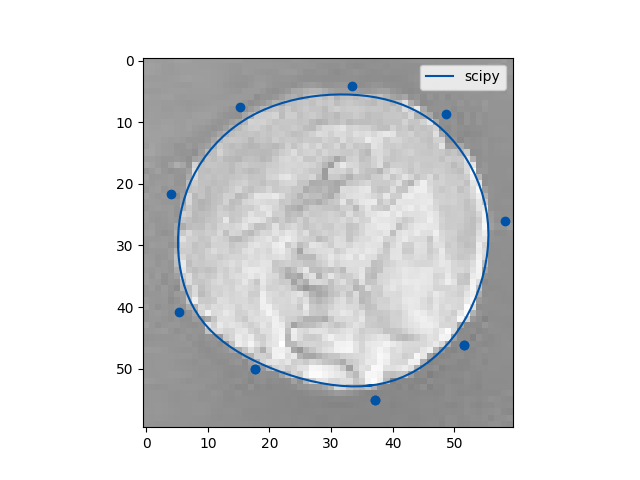
Let see how this compares to scipy…

# Number of data points
N = len(contour)
k = 3

To get a spline with a specific number of control points in scipy we have to precalculate the parameters values t for the knots and the parameter values u for the data points. It is important that we account for the periodicity and padding of the knots.

t = np.arange(-k, M + k + 1)
u = np.linspace(0, M, N + 1)[:-1]

When constructinc the spline using splprep we have to specify the oder of the basis spline, the u and t we just computed, and the periodicity. Since we don’t want to smooth our fit but instead regularize it by fixing the number of control points we need to set s=0 and task=-1.

tck, u = scipy.interpolate.splprep(contour.T, k=k, u=u, t=t, task=-1, s=0, per=N)
ts = np.linspace(0, M, 100)
scipy_vals = scipy.interpolate.splev(ts, tck)
scipy_control_points = tck[1]

plt.imshow(img, cmap="gray", alpha=0.5)
plt.plot(scipy_vals[1], scipy_vals[0], label="scipy", color=scipy_blue)
plt.scatter(scipy_control_points[1], scipy_control_points[0], color=scipy_blue)
plt.legend()
plt.show()