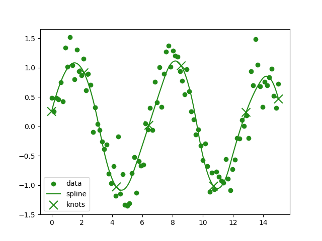
Approximating a Noisy Signal

In this example, we add noise to a sinusoidal signal and then approximate it using an exponential spline.

import matplotlib.pyplot as plt
import numpy as np
import splinebox

We generate example data with 100 points by evaluating a sine function at equidistant points over the interval from 0 to 15. To simulate real-world data, we add Gaussian noise with a standard deviation of 0.3.

N = 100
x = np.linspace(0, 15, N)
values = np.sin(x) + np.random.normal(0, 0.3, N)

To approximate this data, we’ll use an exponential spline, which can effectively model sinusoidal functions. We aim to use the smallest number of knots that still allows the spline to accurately approximate the signal. Empirical testing indicates that 8 knots provide a good balance between simplicity and accuracy in this case.

M = 8
basis_function = splinebox.Exponential(M)
spline = splinebox.Spline(M, basis_function, closed=False)

spline.fit(values)

To plot the spline we evaluate it at finely spaced parameter values.

ts = np.linspace(0, M - 1, 1000)
spline_y = spline(ts)
spline_x = np.linspace(x.min(), x.max(), len(ts))

plt.scatter(x, values, label="data")
plt.plot(spline_x, spline_y, label="spline")
plt.scatter(np.linspace(x.min(), x.max(), M), spline.knots, label="knots", marker="x", sizes=np.ones(M) * 150)
plt.legend()
plt.show()