Fit boundary conditions

Show how changing the boundary conditions affect the fit of a 2D spline.

import matplotlib.pyplot as plt
import numpy as np
import splinebox

We start by creating some random data points generated from a sin curve with noise.

np.random.seed(4)
x = np.sort(np.random.rand(25) * 2 * np.pi)
y = np.sin(x) + np.random.rand(len(x)) * 0.5
data = np.stack([x, y], axis=-1)

To be able to compare the different boundary conditions, we create three separate spline objects and fit each one to the data using a different boundary condition.

M = 5
basis_function = splinebox.B3()
closed = False

free_spline = splinebox.Spline(M, basis_function, closed)
clamped_spline = splinebox.Spline(M, basis_function, closed)
natural_spline = splinebox.Spline(M, basis_function, closed)

free_spline.fit(data, boundary_condition="free")
clamped_spline.fit(data, boundary_condition="clamped")
natural_spline.fit(data, boundary_condition="natural")

We can verify that the first and second derivative are zero for the clamped and natural boundary condition respectively.

print("First derivative at ends of clamped spline")
print(clamped_spline(0, derivative=1))
print(clamped_spline(M - 1, derivative=1))

print("Second derivative at ends of natural spline")
print(natural_spline(0, derivative=2))
print(natural_spline(M - 1, derivative=2))

First derivative at ends of clamped spline
[0. 0.]
[0. 0.]
Second derivative at ends of natural spline
[0. 0.]
[0. 0.]

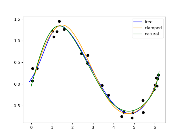
Lastly, we plot the splines to see how the splines differ.

t = np.linspace(0, M - 1, 1000)
free_points = free_spline(t)
clamped_points = clamped_spline(t)
natural_points = natural_spline(t)

plt.scatter(data[:, 0], data[:, 1], color="black")
plt.plot(free_points[:, 0], free_points[:, 1], label="free", color="blue")
plt.plot(clamped_points[:, 0], clamped_points[:, 1], label="clamped", color="orange")
plt.plot(natural_points[:, 0], natural_points[:, 1], label="natural", color="green")
plt.legend()
plt.show()

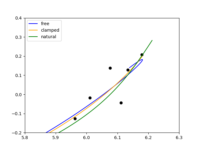
Zooming in on the right end of the spline, reveals that the spline with free boundary conditions exhibits an undesired sharp curve.

plt.scatter(data[:, 0], data[:, 1], color="black")
plt.plot(free_points[:, 0], free_points[:, 1], label="free", color="blue")
plt.plot(clamped_points[:, 0], clamped_points[:, 1], label="clamped", color="orange")
plt.plot(natural_points[:, 0], natural_points[:, 1], label="natural", color="green")
plt.xlim(5.8, 6.3)
plt.ylim(-0.2, 0.4)
plt.legend()
plt.show()