Multivariate splines

This example demonstrates the multivariate spline capabilities of SplineBox. A multivariate spline is a tensor product of univariate splines: it takes nvariate parameters and returns a value in a (possibly multi-dimensional) codomain. The control points are simply a NumPy array whose first nvariate axes form the control grid and whose last axis contains the codomain values.

import matplotlib.pyplot as plt
import numpy as np
import pyvista

import splinebox
import splinebox.multivariate

Bivariate scalar surface

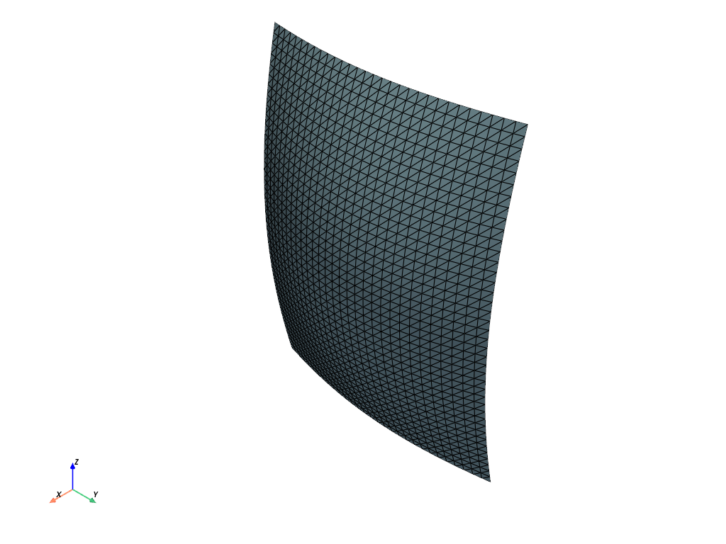
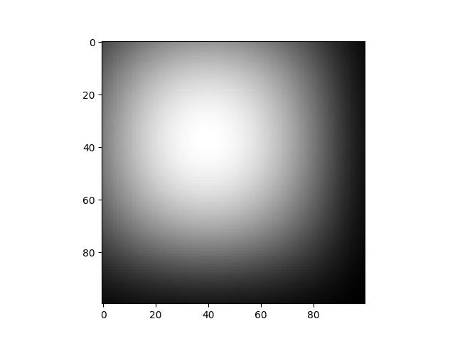
A bivariate spline takes two parameters and returns a scalar. We build the control-point array directly and visualize the resulting surface.

M = (4, 5)
closed = (False, False)

spline = splinebox.multivariate.MultivariateSpline(M=M, basis_functions=splinebox.B3(), closed=closed)

# For an open B3 spline the control grid is padded by one point on each side.
control_points = np.zeros((M[0] + 2 * spline.pad[0], M[1] + 2 * spline.pad[1], 1))
# Place a bump in the middle of the control grid.
control_points[2:4, 2:5, 0] = 1.0
spline.control_points = control_points

# Evaluate on a dense grid.
t = np.stack(
    np.meshgrid(*(np.linspace(0, m - 1, 100) for m in M), indexing="ij"),
    axis=-1,
)
vals = spline(t)

fig, ax = plt.subplots()
ax.imshow(vals, origin="lower")
ax.set_title("Bivariate scalar surface")
plt.show()

# The same surface can be exported as a PyVista mesh.
points, connectivity = spline.mesh()
connectivity = np.hstack((np.full((connectivity.shape[0], 1), 3), connectivity))
mesh = pyvista.PolyData(points, faces=connectivity)
mesh.plot(show_edges=True)

Static Scene

Interactive Scene

Bivariate 3-D surface: a pipe

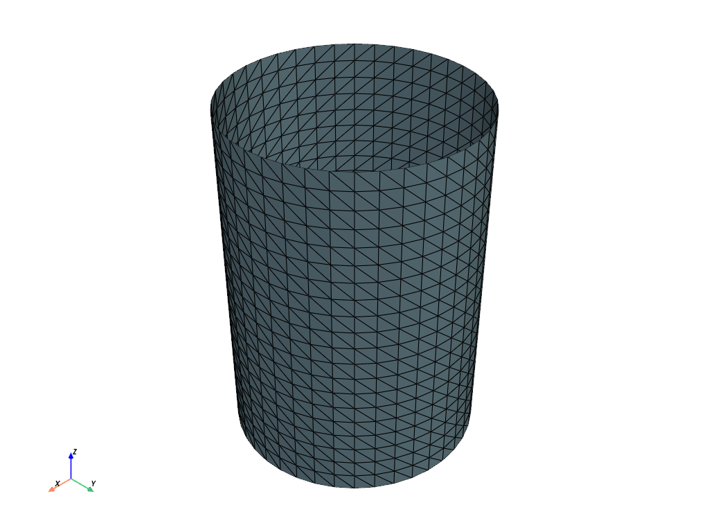
A bivariate spline can also map two parameters to 3-D points. Here we build a pipe that is closed around its circumference and open along its axis. The control points are constructed directly from a circular profile and an extrusion axis. splinebox.multivariate.tensor_product() is one way to obtain the same array when the geometry is separable.

M = (4, 3)
closed = (True, False)

# Exponential basis for a smooth closed cross-section, B1 for a linear axis.
basis_functions = (splinebox.Exponential(M[0]), splinebox.B1())

# Circular profile in the x-y plane.
phi = np.linspace(0, 2 * np.pi, M[0], endpoint=False)
x_circle = np.sin(phi) + 3
y_circle = np.cos(phi) - 2

# Extrusion axis along z.
z_axis = np.array([0, 1, 2]) + 5

# Direct construction of the control-point array.
control_points = np.empty((M[0], M[1], 3))
control_points[..., 0] = x_circle[:, None]
control_points[..., 1] = y_circle[:, None]
control_points[..., 2] = z_axis[None, :]

# Equivalent separable construction using tensor_product:
# profile = np.stack([x_circle, y_circle, np.ones(M[0])], axis=-1)
# axis = np.stack([np.ones(M[1]), np.ones(M[1]), z_axis], axis=-1)
# control_points = splinebox.multivariate.tensor_product([profile, axis])

spline = splinebox.multivariate.MultivariateSpline(
    M=M, basis_functions=basis_functions, closed=closed, control_points=control_points
)

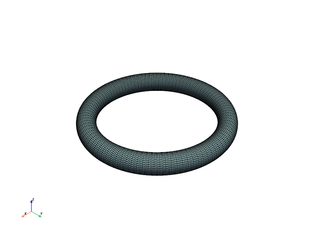
points, connectivity = spline.mesh()
connectivity = np.hstack((np.full((connectivity.shape[0], 1), 3), connectivity))
mesh = pyvista.PolyData(points, faces=connectivity)
mesh.plot(show_edges=True)

Static Scene

Interactive Scene

Fitting a spline to data

MultivariateSpline.fit finds control points that approximate a given scalar or vector field. Below we sample a smooth scalar function on a coarse grid, add noise, and fit a B3 spline with fewer knots than data points.

M = (6, 6)
fit_spline = splinebox.multivariate.MultivariateSpline(M=M, basis_functions=splinebox.B3(), closed=(False, False))

# Coarse noisy observations.
data_shape = (20, 20)
t_data = np.stack(
    np.meshgrid(
        np.linspace(0, M[0] - 1, data_shape[0]),
        np.linspace(0, M[1] - 1, data_shape[1]),
        indexing="ij",
    ),
    axis=-1,
)
X, Y = t_data[..., 0], t_data[..., 1]
true_values = np.sin(X) * np.cos(Y)
noisy_values = true_values + 0.2 * np.random.randn(*data_shape)

fit_spline.fit(noisy_values, t=t_data)

# Evaluate the fit on a fine grid.
t_fine = np.stack(
    np.meshgrid(np.linspace(0, M[0] - 1, 100), np.linspace(0, M[1] - 1, 100), indexing="ij"),
    axis=-1,
)
fit_values = fit_spline(t_fine).squeeze()

fig, axes = plt.subplots(1, 3, figsize=(12, 4))
for ax, data, title in [
    (axes[0], true_values, "True function"),
    (axes[1], noisy_values, "Noisy data"),
    (axes[2], fit_values, "Fitted spline"),
]:
    im = ax.imshow(data, origin="lower")
    ax.set_title(title)
    fig.colorbar(im, ax=ax, shrink=0.6)
plt.tight_layout()
plt.show()

Trivariate spline

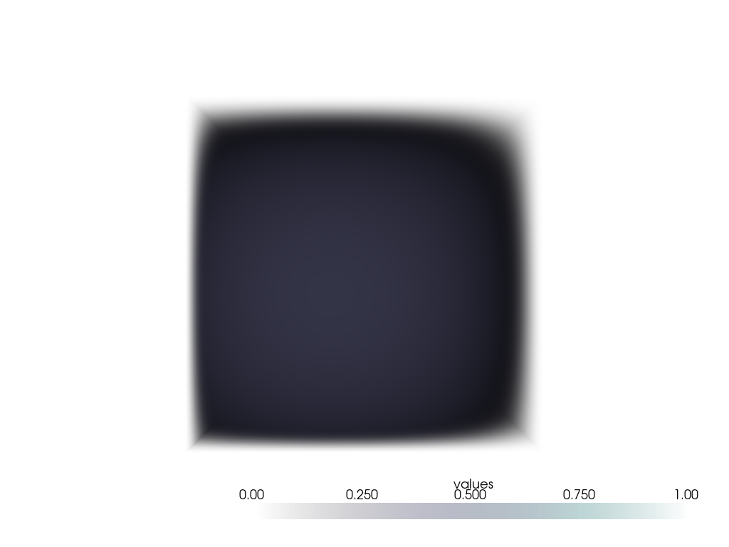
A trivariate spline has three parameter dimensions and can represent a scalar or vector volume.

trivariate_M = (5, 5, 5)
trivariate_closed = (False, False, False)
trivariate_basis_functions = splinebox.B3()

# For an open B3 spline each dimension is padded by one point on each side.
control_points = np.zeros((7, 7, 7, 1))
# Place a spherical blob near the centre of the control grid.
centre = np.array([3.0, 3.0, 3.0])
for i in range(7):
    for j in range(7):
        for k in range(7):
            if np.linalg.norm(np.array([i, j, k]) - centre) < 1.5:
                control_points[i, j, k, 0] = 1.0

spline = splinebox.multivariate.MultivariateSpline(
    M=trivariate_M,
    basis_functions=trivariate_basis_functions,
    closed=trivariate_closed,
    control_points=control_points,
)

t = np.stack(
    np.meshgrid(
        *(np.linspace(0, m - 1, 30) for m in trivariate_M),
        indexing="ij",
    ),
    axis=-1,
)
vals = spline(t).squeeze()

grid = pyvista.ImageData(dimensions=np.array(vals.shape) + 1)
grid.origin = (0, 0, 0)
grid.spacing = (1, 1, 1)
grid.cell_data["values"] = vals.flatten(order="F")
plotter = pyvista.Plotter()
plotter.add_volume(grid, cmap="bone", clim=(0, 1))
plotter.camera_position = "yz"
plotter.show()

Static Scene

Interactive Scene