Note
Go to the end to download the full example code.
Performance comparison with scipy#
In this example we will compare splinebox’s performance to scipy’s splines on the following three tasks:
Spline creation
Spline evalution
Data fitting
import time

import matplotlib.pyplot as plt
import numpy as np
import pandas as pd
import scipy
import seaborn as sns
import splinebox
First we compare the time it takes to create spline with a given set of knots and to evalutate it. The measurement is repeated 11 and the first repretition is discarded, because of the necessary numba compilation. The compiled code is cached such that it can be reused for future runs. Times are computes for different numbers of knots (M), open and closed splines, and curves with different dimensionality.
n_repetitions = 10

Ms = np.arange(10, 101, 10)

results_creation = []
results_evaluation = []

for closed in [True, False]:
    for ndim in (1, 2, 3, 10):
        for M in Ms:
            for repetition in range(n_repetitions + 1):
                knots = np.random.rand(M, ndim)

                start = time.perf_counter_ns()
                spline = splinebox.Spline(M, splinebox.B3(), closed=closed)
                spline.knots = knots
                stop = time.perf_counter_ns()
                if repetition != 0:
                    results_creation.append(
                        [
                            "splinebox",
                            f"{ndim}D",
                            M,
                            "closed" if closed else "open",
                            stop - start,
                        ]
                    )

                for nt in [10, 100, 1000, 10000]:
                    t = np.linspace(0, M if closed else M - 1, nt)
                    start_eval = time.perf_counter_ns()
                    spline.eval(t)
                    stop_eval = time.perf_counter_ns()
                    if repetition != 0:
                        results_evaluation.append(
                            [
                                "splinebox",
                                f"{ndim}D",
                                M,
                                nt,
                                "closed" if closed else "open",
                                stop - start,
                            ]
                        )

                if closed:
                    start = time.perf_counter_ns()
                    t_knots = np.arange(M + 1)
                    knots_periodic = np.concatenate([knots, knots[0][np.newaxis, :]], axis=0)
                    spline = scipy.interpolate.make_interp_spline(t_knots, knots_periodic, k=3, bc_type="periodic")
                    stop = time.perf_counter_ns()
                else:
                    start = time.perf_counter_ns()
                    t_knots = np.arange(M)
                    spline = scipy.interpolate.make_interp_spline(t_knots, knots, k=3, bc_type="natural")
                    stop = time.perf_counter_ns()

                if repetition != 0:
                    results_creation.append(
                        [
                            "scipy",
                            f"{ndim}D",
                            M,
                            "closed" if closed else "open",
                            stop - start,
                        ]
                    )

                for nt in [10, 100, 1000, 10000]:
                    t = np.linspace(0, M if closed else M - 1, nt)
                    start_eval = time.perf_counter_ns()
                    spline(t)
                    stop_eval = time.perf_counter_ns()
                    if repetition != 0:
                        results_evaluation.append(
                            [
                                "scipy",
                                f"{ndim}D",
                                M,
                                nt,
                                "closed" if closed else "open",
                                stop - start,
                            ]
                        )
Now, that we have collected all of the times, we can turn the results into a data frame and plot the results using seaborn.
df = pd.DataFrame(results_creation, columns=["Package", "Dimensionality", "Number of knots", "closed", "time [ns]"])
for periodicity in ["closed", "open"]:
    fig, ax = plt.subplots()
    ax.set(yscale="log")
    sns.set_palette(sns.color_palette(["#228b18", "#0053a6"]))
    sns.lineplot(
        x="Number of knots",
        y="time [ns]",
        hue="Package",
        style="Dimensionality",
        data=df.loc[df["closed"] == periodicity],
        ax=ax,
    )
    plt.title(f"Creation of {periodicity} splines")
    plt.show()
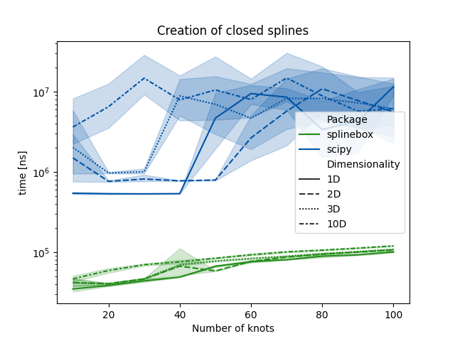
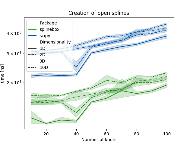
The results show that splinbox outperforms scipy in all condition for the task of creating a spline from a given set of knots.
df = pd.DataFrame(
    results_evaluation,
    columns=["Package", "Dimensionality", "Number of knots", "Number of parameter values", "closed", "time [ns]"],
)
for periodicity in ["closed", "open"]:
    fig, ax = plt.subplots(figsize=(7, 7))
    ax.set(yscale="log")
    sns.set_palette(sns.color_palette(["#228b18", "#0053a6"]))
    sns.lineplot(
        x="Number of knots",
        y="time [ns]",
        hue="Package",
        style="Number of parameter values",
        data=df.loc[df["closed"] == periodicity],
        ax=ax,
    )
    plt.title(f"Evaluation of {periodicity} splines")
    plt.show()
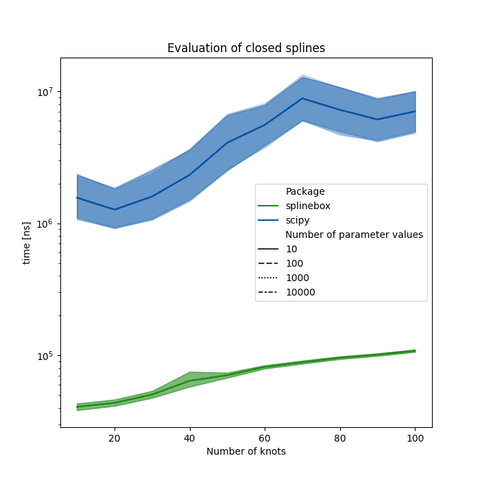
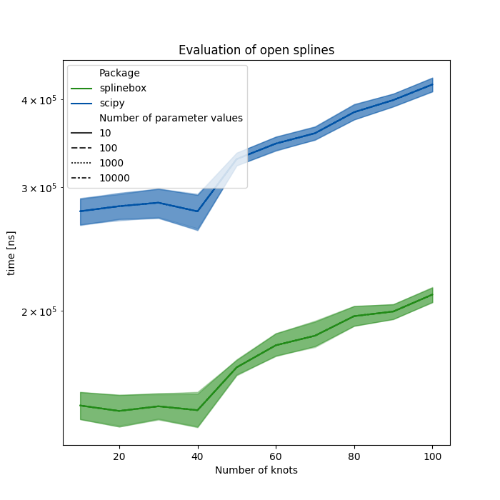
Once again, splinebox outperforms scipy, in all conditions for the spline evaluation task. Lastly, we will compare the fitting (i.e. determining the control points of spline with M knots using least-squares given N > M datapoints) performance.
results_fitting = []
for closed in [True, False]:
    for ndim in (1, 2, 3, 10):
        for M in Ms:
            for repetition in range(n_repetitions + 1):
                data = np.random.rand(M * 10, ndim)

                start = time.perf_counter_ns()
                spline = splinebox.Spline(M, splinebox.B3(), closed=closed)
                spline.fit(data)
                stop = time.perf_counter_ns()

                if repetition != 0:
                    results_fitting.append(
                        [
                            "splinebox",
                            f"{ndim}D",
                            M,
                            "closed" if closed else "open",
                            stop - start,
                        ]
                    )

                k = 3
                if closed:
                    start = time.perf_counter_ns()
                    N = len(data)
                    t = np.arange(-k, M + k + 1)
                    u = np.linspace(0, M, N + 1)[:-1]
                    tck, u = scipy.interpolate.splprep(data.T, k=k, u=u, t=t, task=-1, s=0, per=N)
                    stop = time.perf_counter_ns()

                else:
                    start = time.perf_counter_ns()
                    N = len(data)
                    t = np.arange(-k, M + k)
                    u = np.linspace(0, M - 1, N)
                    tck, u = scipy.interpolate.splprep(data.T, k=k, u=u, t=t, task=-1, s=0)
                    stop = time.perf_counter_ns()

                if repetition != 0:
                    results_fitting.append(
                        [
                            "scipy",
                            f"{ndim}D",
                            M,
                            "closed" if closed else "open",
                            stop - start,
                        ]
                    )
df = pd.DataFrame(
    results_fitting,
    columns=["Package", "Dimensionality", "Number of knots", "closed", "time [ns]"],
)
for periodicity in ["closed", "open"]:
    fig, ax = plt.subplots(figsize=(7, 7))
    ax.set(yscale="log")
    sns.set_palette(sns.color_palette(["#228b18", "#0053a6"]))
    sns.lineplot(
        x="Number of knots",
        y="time [ns]",
        hue="Package",
        style="Dimensionality",
        data=df.loc[df["closed"] == periodicity],
        ax=ax,
    )
    plt.title(f"Fitting of {periodicity} splines")
    plt.show()
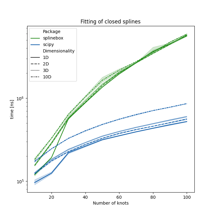
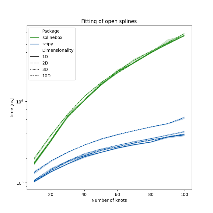
In the fitting task splinebox is outperformed by scipy’s splprep, but is competetive for splines with relatively few knots (i.e. < 20).
Total running time of the script: (0 minutes 28.598 seconds)