Active Contours

This example demonstrates a basic active contours (snakes) implementation using splinebox. The goal is to segment the astronaut’s head in an image by iteratively refining a spline contour.

import matplotlib
import matplotlib.pyplot as plt
import numpy as np
import scipy
import skimage
import splinebox.basis_functions
import splinebox.spline_curves

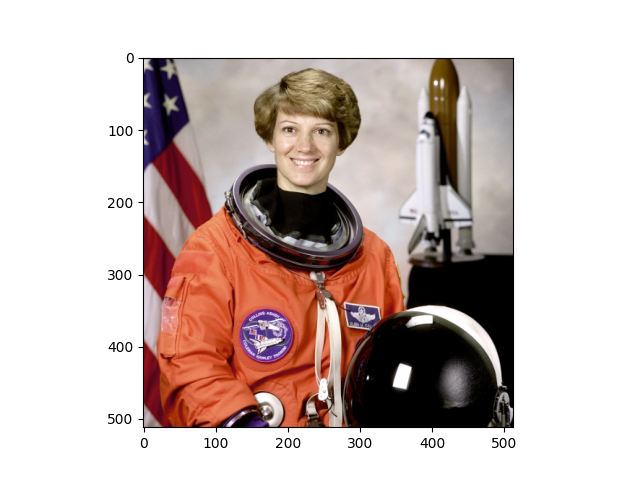
Let’s load the astronaut example image from skimage.

img = skimage.data.astronaut()

plt.imshow(img)
plt.show()

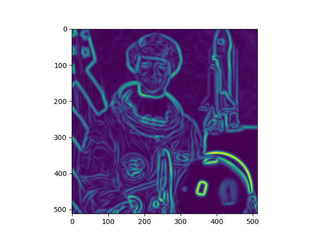
To make the contour stick to the edges of the image, we compute an edge map. First, convert the image to grayscale, apply Gaussian smoothing to reduce noise, and then apply the Sobel filter for edge detection.

gray = skimage.color.rgb2gray(img)
smooth = skimage.filters.gaussian(gray, 3, preserve_range=False)
edge = skimage.filters.sobel(smooth)

plt.imshow(edge)
plt.show()

To make calculating the edge energy at non-integer locations easier, we use a surface spline on a regular grid. This returns a callable object that can be queried for edge energy values.

edge_energy = scipy.interpolate.RectBivariateSpline(
    np.arange(edge.shape[1]), np.arange(edge.shape[0]), edge, kx=2, ky=2, s=1
)

We define an internal energy function to regularize the curvature of the spline. The internal energy depends on the first and second derivatives of the spline.

def internal_energy(spline, t, alpha, beta):
    return 0.5 * (alpha * spline(t, derivative=1) ** 2 + beta * spline(t, derivative=2) ** 2)

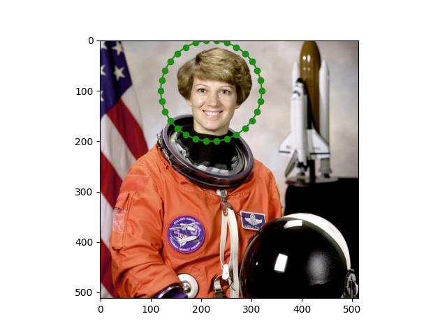
Initialize the spline with 30 knots that form a circle around the astronaut’s head.

M = 30
s = np.linspace(0, 2 * np.pi, M + 1)[:-1]
y = 100 + 100 * np.sin(s)
x = 220 + 100 * np.cos(s)
knots = np.array([y, x]).T

We keep a copy of the initial knots so we can plot them later.

initial_knots = knots.copy()

Now, we can construct a B3 spline and set its control points (coefficients) using the knots we generated above.

spline = splinebox.spline_curves.Spline(M=M, basis_function=splinebox.basis_functions.B3(), closed=True)
spline.knots = knots

t = np.linspace(0, M, 400)
contour = spline(t)
plt.imshow(img)
plt.scatter(knots[:, 1], knots[:, 0])
plt.plot(contour[:, 1], contour[:, 0])
plt.show()

Here, we set the necessary paramters for the active contours algorithm:

• \(\alpha\) controls the contribution of the first derivative (smoothness) to the internal energy

• \(\beta\) controls the contribution of the second derivative (curvature) to the internal energy

alpha = 0
beta = 0.001

# Store intermediate contours
contours = []
# Store the energy values
external_energies = []

Nex, we define the energy function to be minimized. It combines the external energy from the edge map and the internal energy based on spline smoothness and curvature.

def energy_function(control_points, spline, t, alpha, beta):
    control_points = control_points.reshape((spline.M, -1))
    spline.control_points = control_points
    contour = spline(t)
    contours.append(contour.copy())

    # Compute external energy from the edge map
    edge_energy_value = np.sum(edge_energy(contour[:, 0], contour[:, 1], grid=False))
    external_energies.append(-edge_energy_value)

    # Compute internal energy
    internal_energy_value = np.sum(internal_energy(spline, t, alpha, beta))

    # Total energy to minimize
    return -edge_energy_value + internal_energy_value

The active contours approach consists of iteratively updating our control points (coefficients) to minimize the energy and find the optimal contour.

initial_control_points = spline.control_points.copy()
result = scipy.optimize.minimize(
    energy_function, initial_control_points.flatten(), method="Powell", args=(spline, t, alpha, beta)
)

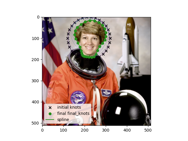
Inorder to plot the spline as a smooth line, we have to evaluate it more densly than just at the knots.

samples = spline(t)

final_knots = spline(np.arange(M))

Finaly, we can plot the result.

plt.imshow(img)
plt.scatter(initial_knots[:, 1], initial_knots[:, 0], marker="x", color="black", label="initial knots")
contours = contours[::2000]
colors = matplotlib.colormaps["viridis"](np.linspace(0, 1, len(contours)))
for contour, color in zip(contours, colors):
    plt.plot(contour[:, 1], contour[:, 0], color=color, alpha=0.2)
plt.scatter(final_knots[:, 1], final_knots[:, 0], marker="o", label="final final_knots")
plt.plot(samples[:, 1], samples[:, 0], label="spline")
plt.legend()
plt.show()