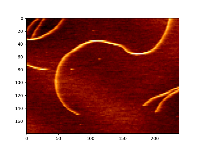
Measure the curvature of a peptide

In this example, we measure the curvature of a peptide in an AFM image.

Image credit: Yiwei Zheng, LBNI, EPFL

import matplotlib.pyplot as plt
import numpy as np
import scipy
import skan
import skimage
import splinebox
import tifffile

1. Load and Inspect the Data

img = tifffile.imread("peptides.tif")

plt.imshow(img, cmap="afmhot")
plt.show()

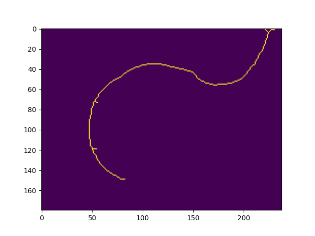
2. Segmentation and Skeletonization

thresh = skimage.filters.threshold_otsu(img)
mask = img > thresh
skeleton = skimage.morphology.skeletonize(mask)
label_img = skimage.measure.label(skeleton)
label_biggest = np.argmax(np.bincount(label_img.flatten())[1:]) + 1
skeleton = label_img == label_biggest

plt.imshow(skeleton)
plt.show()

3. Select longest path

graph, coords = skan.csr.skeleton_to_csgraph(skeleton)
coords = np.stack(coords, axis=-1)

dist_matrix, predecessors = scipy.sparse.csgraph.shortest_path(graph, return_predecessors=True)
stop_index, start_index = np.unravel_index(np.argmax(dist_matrix), dist_matrix.shape)
i = start_index
skeleton_points = []
while i != stop_index:
    skeleton_points.append(coords[i])
    i = predecessors[stop_index, i]
skeleton_points = np.array(skeleton_points)

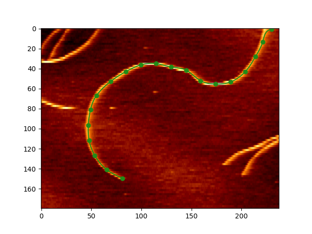
4. Fit Spline

M = 20
basis_function = splinebox.basis_functions.B3()
initial_spline = splinebox.spline_curves.Spline(M=M, basis_function=basis_function, closed=False)
initial_spline.fit(skeleton_points)

t = np.linspace(0, M - 1, M * 100)
initial_vals = initial_spline(t)
initial_knots = initial_spline.knots

plt.imshow(img, cmap="afmhot")
plt.plot(initial_vals[:, 1], initial_vals[:, 0])
plt.scatter(initial_knots[:, 1], initial_knots[:, 0])
plt.show()

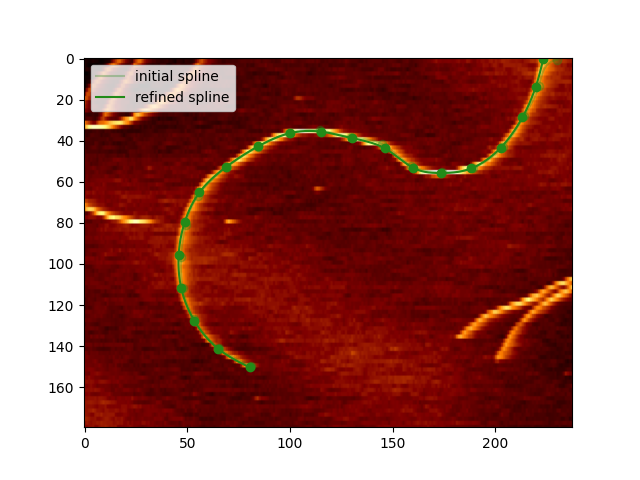
5. Refine Spline

def loss_function(control_points, alpha):
    spline.control_points = control_points.reshape((-1, 2))
    coords = spline(t)
    pixel_values = scipy.ndimage.map_coordinates(img, coords.T)
    image_energy = np.mean(pixel_values)
    internal_energy = np.mean(spline(t, derivative=2) ** 2)
    energy = -1 * image_energy + alpha * internal_energy
    return energy


initial_control_points = initial_spline.control_points
spline = initial_spline.copy()
scipy.optimize.minimize(
    loss_function,
    initial_control_points.flatten(),
    args=(0.3,),
    method="Powell",
    tol=0.01,
)

vals = spline(t)
knots = spline.knots

plt.figure()
plt.imshow(img, cmap="afmhot")
plt.plot(initial_vals[:, 1], initial_vals[:, 0], label="initial spline", alpha=0.3)
plt.scatter(initial_knots[:, 1], initial_knots[:, 0], alpha=0.3)
plt.plot(vals[:, 1], vals[:, 0], label="refined spline")
plt.scatter(knots[:, 1], knots[:, 0])
plt.legend()
plt.show()

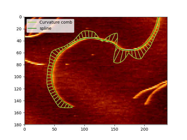
6. Curvature Comb

total_length = spline.arc_length()
lengths = np.linspace(0, total_length, 200)
t = spline.arc_length_to_parameter(lengths)

vals = spline(t)
curvature = spline.curvature(t)
normals = spline.normal(t)

comb = vals + 500 * curvature[:, np.newaxis] * normals

plt.figure()
plt.imshow(img, cmap="afmhot")
plt.plot(comb[:, 1], comb[:, 0], label="Curvature comb", color="yellowgreen")
for p in range(0, len(t), 3):
    plt.plot([vals[p, 1], comb[p, 1]], [vals[p, 0], comb[p, 0]], color="yellowgreen")
plt.plot(vals[:, 1], vals[:, 0], label="spline")
plt.xlim((0, img.shape[1]))
plt.ylim((img.shape[0], 0))
plt.legend()
plt.show()

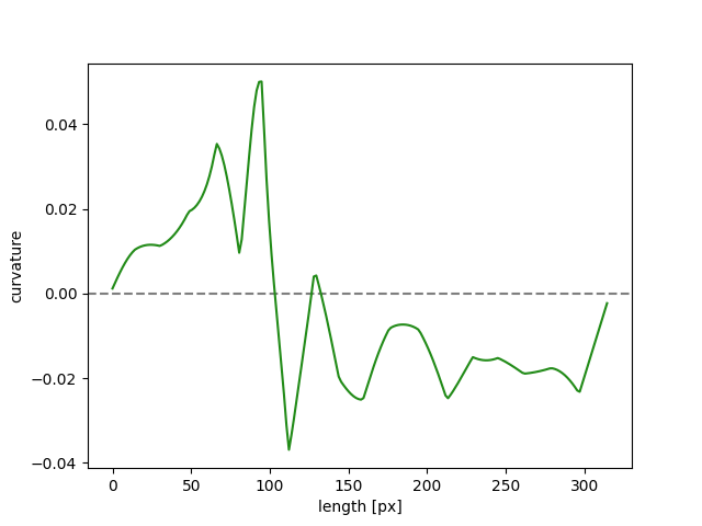
7. Plot Curvature vs. Length

plt.figure()
plt.axhline(0, linestyle="--", color="black", alpha=0.5)
plt.plot(lengths, curvature)
plt.xlabel("length [px]")
plt.ylabel("curvature")
plt.show()