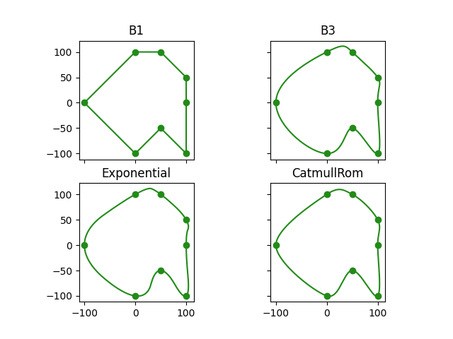
Closed interpolating splines

This example demonstrates how the choice of basis function influences the shape of a spline. We use a fixed set of knots and construct splines using different basis functions to observe their effects.

import matplotlib.pyplot as plt
import numpy as np
import splinebox.basis_functions
import splinebox.spline_curves

We define a set of arbitrary 2D points as knots.

knots = np.array([[0, 100], [50, 100], [100, 50], [100, 0], [100, -100], [50, -50], [0, -100], [-100, 0]])

We define the parameter values to evaluate the spline for plotting.

t = np.linspace(0, len(knots), 1000)

Set up a grid of subplots for visual comparison of different basis functions and loop through different basis functions to construct the corresponding splines and plot them.

n, m = 2, 2
fig, axes = plt.subplots(n, m, sharex=True, sharey=True)

for i, (name, basis_function) in enumerate(
    (
        ("B1", splinebox.basis_functions.B1()),
        ("B3", splinebox.basis_functions.B3()),
        ("Exponential", splinebox.basis_functions.Exponential(len(knots))),
        ("CatmullRom", splinebox.basis_functions.CatmullRom()),
    )
):
    M = len(knots)
    curve = splinebox.spline_curves.Spline(M, basis_function, True)
    curve.knots = knots
    discreteContour = curve(t)

    axes[i // n, i % n].scatter(knots[:, 0], knots[:, 1])
    axes[i // n, i % n].plot(discreteContour[:, 0], discreteContour[:, 1])
    axes[i // n, i % n].set_title(name)
    axes[i // n, i % n].set_aspect("equal", adjustable="box")

plt.show()