Multivariate splines

This example demonstrates how to create multivariate splines using SplineBox.

import matplotlib.pyplot as plt
import numpy as np
import pyvista
import splinebox
import splinebox.multivariate

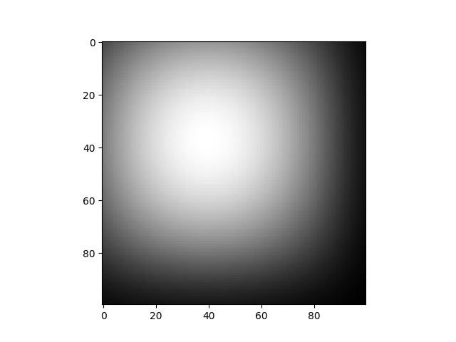
1. 1D Bivariate surface spline

1D Bivariate surface spline is a spline that takes two parameters and returns a scalar.

M = (4, 5)
closed = (False, False)
control_points = splinebox.multivariate.tensor_product([np.sin(np.linspace(0, np.pi, m + 2)) for m in M])

spline = splinebox.multivariate.MultivariateSpline(
    M=M, basis_functions=splinebox.B3(), closed=closed, control_points=control_points
)

t = np.stack(np.meshgrid(*(np.linspace(0, m, 100) for m in M), indexing="ij"), axis=-1)

vals = spline(t)

plt.imshow(vals)
plt.show()

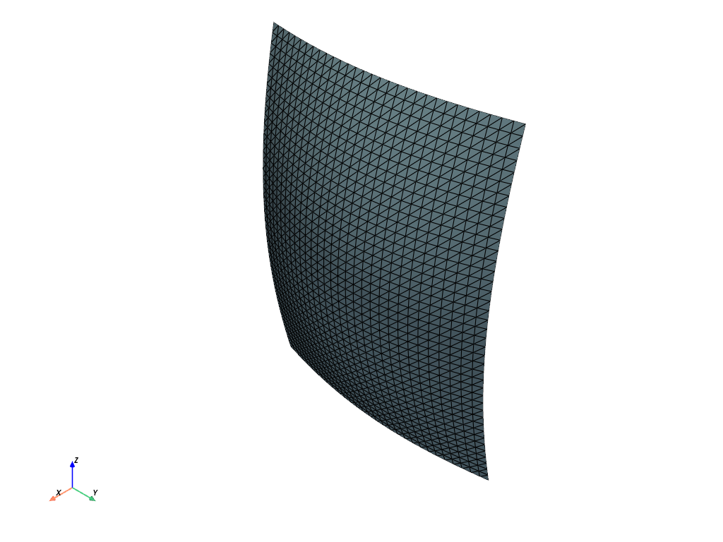
points, connectivity = spline.mesh()

# Prepend the number of points in each element (3 for triangles) for PyVista
connectivity = np.hstack((np.full((connectivity.shape[0], 1), 3), connectivity))

# Create and plot the PyVista mesh
mesh = pyvista.PolyData(points, faces=connectivity)
mesh.plot(show_edges=True)

Static Scene

Interactive Scene

2. 3D Bivariate surface spline

3D Bivariate surface spline is a spline that takes two parameters and returns a 3D vector. As an example we will create a pipe shaped surface.

M = (4, 3)
closed = (True, False)

We want the spline to be circular in one direction and straight in the other. For the circular direction we choose an exponential basis function and for the straight direction we choose the B1 basis function.

basis_functions = (splinebox.Exponential(M[0]), splinebox.B1())

Let’s create the control points for the circular direction. We create four points equally spaced on a circle with radius one in the x-y plane. Note that we have to set z to one and not zeros because the control points are multiplied in a multivariate spline and not added.

x = np.sin(np.linspace(0, 2 * np.pi, M[0] + 1))[:-1] + 3
y = np.cos(np.linspace(0, 2 * np.pi, M[0] + 1))[:-1] - 2
z = np.ones(M[0])
control_points_circular = np.stack([x, y, z], axis=-1)

Next, we construct the control points for the straight direction.

x = np.ones(M[1])
y = np.ones(M[1])
# x = np.array([0.5, 1, 0.5])
# y = np.array([1, 0.5, 1])
# x = np.array([1, 1, 0.5])
# y = np.array([1, 0.5, 1])
z = np.array([0, 1, 2]) + 5
control_points_straight = np.stack([x, y, z], axis=-1)

control_points = splinebox.multivariate.tensor_product([control_points_circular, control_points_straight])

spline = splinebox.multivariate.MultivariateSpline(
    M=M, basis_functions=basis_functions, closed=closed, control_points=control_points
)

points, connectivity = spline.mesh()

# Prepend the number of points in each element (3 for triangles) for PyVista
connectivity = np.hstack((np.full((connectivity.shape[0], 1), 3), connectivity))

# Create and plot the PyVista mesh
mesh = pyvista.PolyData(points, faces=connectivity)
mesh.plot(show_edges=True)

Static Scene

Interactive Scene

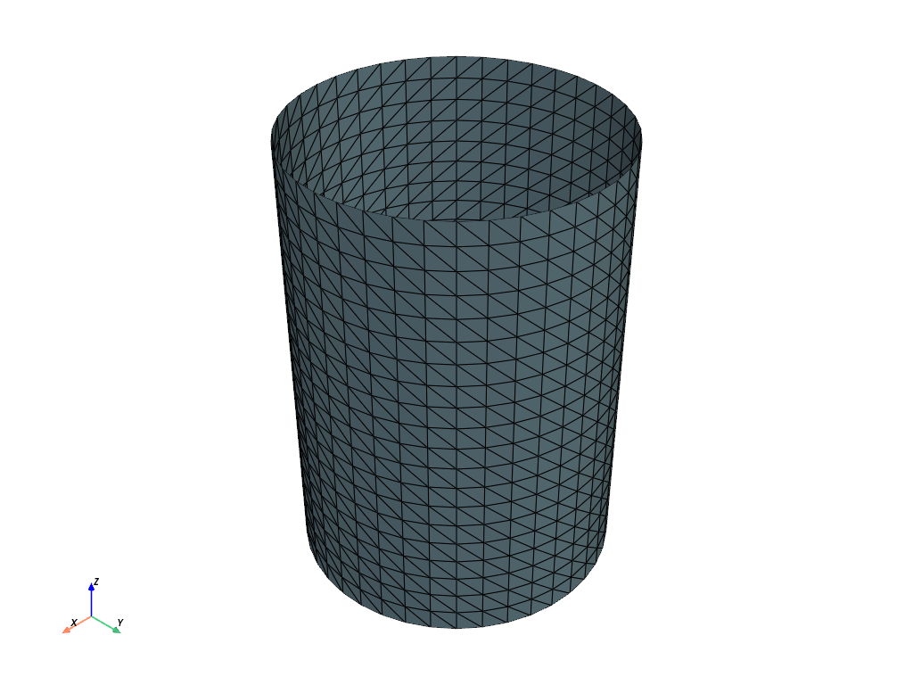
Aligning the pipe along one of the z-axis, allowed us to factorize the element-wise multiplication as follows: $vec[x, y, z] = vec[x, y, 1] * vec[1, 1, z]$

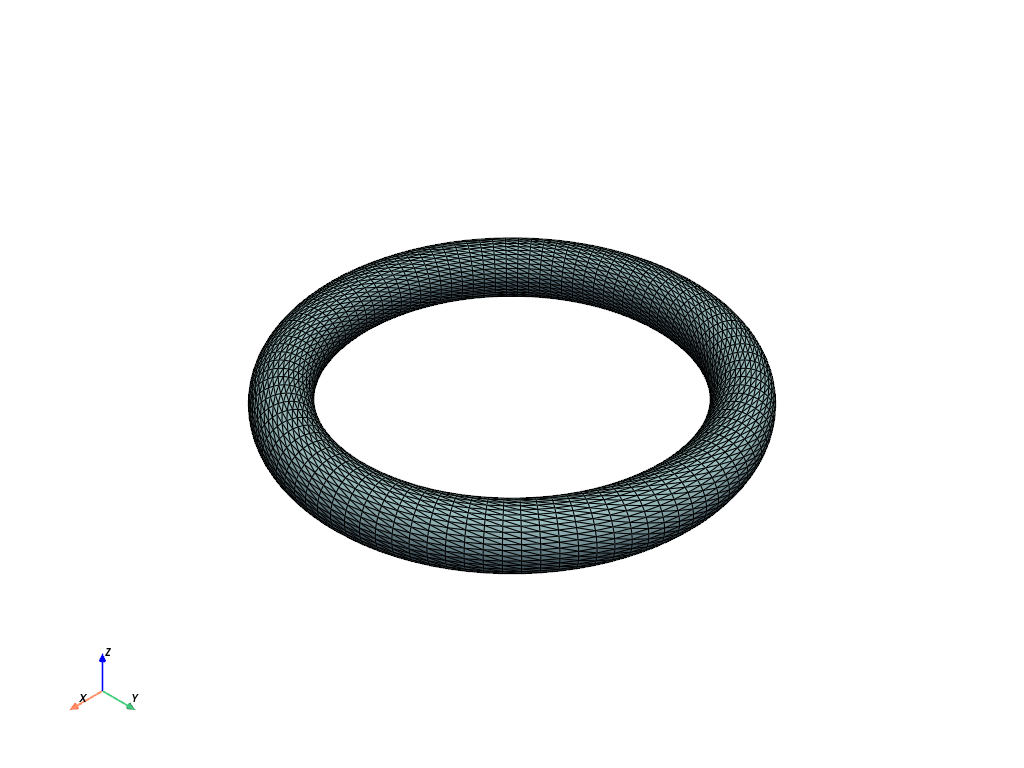
3. The torus

M = (10, 4)
closed = (True, True)
torus_basis_functions = (splinebox.Exponential(M[0]), splinebox.Exponential(M[1]))

R = 5
r = 1
control_points = []
x = np.cos(np.linspace(0, 2 * np.pi, M[0] + 1))[:-1]
y = np.sin(np.linspace(0, 2 * np.pi, M[0] + 1))[:-1]
z = np.ones(M[0])
points = np.stack([x, y, z], axis=-1)
control_points.append(points)
x = r * np.sin(np.linspace(0, 2 * np.pi, M[1] + 1))[:-1] + R
y = r * np.sin(np.linspace(0, 2 * np.pi, M[1] + 1))[:-1] + R
z = r * np.cos(np.linspace(0, 2 * np.pi, M[1] + 1))[:-1]
points = np.stack([x, y, z], axis=-1)
control_points.append(points)
control_points = splinebox.multivariate.tensor_product(control_points)

spline = splinebox.multivariate.MultivariateSpline(
    M=M, basis_functions=torus_basis_functions, closed=closed, control_points=control_points
)

points, connectivity = spline.mesh()

# Prepend the number of points in each element (3 for triangles) for PyVista
connectivity = np.hstack((np.full((connectivity.shape[0], 1), 3), connectivity))

# Create and plot the PyVista mesh
mesh = pyvista.PolyData(points, faces=connectivity)
mesh.plot(show_edges=True)

Static Scene

Interactive Scene

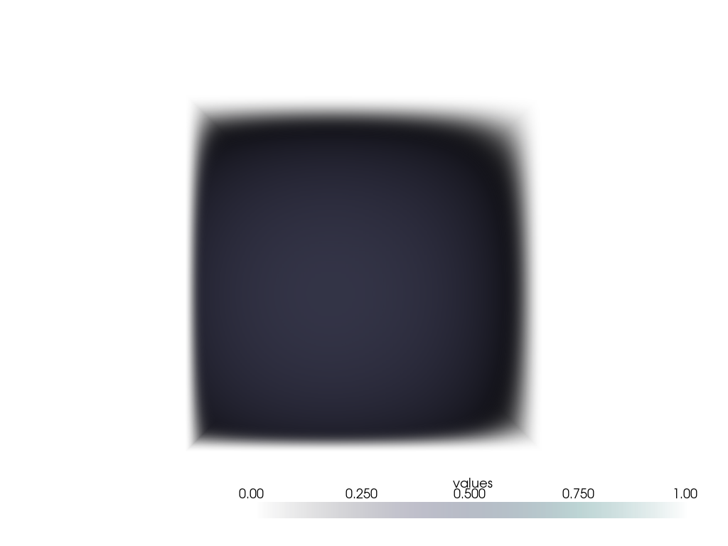
Trivariate spline

trivariate_M = (7, 5, 8)
trivariate_closed = (False, False, False)
trivariate_basis_functions = splinebox.B3()
trivariate_control_points = splinebox.multivariate.tensor_product(
    [np.sin(np.linspace(0, np.pi, m + 2)) for m in trivariate_M]
)

spline = splinebox.multivariate.MultivariateSpline(
    M=trivariate_M,
    basis_functions=trivariate_basis_functions,
    closed=trivariate_closed,
    control_points=trivariate_control_points,
)

t = np.stack(np.meshgrid(*(np.linspace(0, m, 100) for m in trivariate_M), indexing="ij"), axis=-1)

vals = spline(t)
vals = np.squeeze(vals)

grid = pyvista.ImageData(dimensions=np.array(vals.shape) + 1)
grid.origin = (0, 0, 0)
grid.spacing = (1, 1, 1)
grid.cell_data["values"] = vals.flatten(order="F")
plotter = pyvista.Plotter()
plotter.add_volume(grid, cmap="bone", clim=(0, 1))
plotter.camera_position = "yz"
plotter.show()

Static Scene

Interactive Scene