Dendrite-Centric Coordinate System

This example demonstrates how to fit a spline to a dendrite and align the image coordinate system with the spline.

Data Source: DeepD3 Data Used: Crop of DeepD3_Benchmark.tif

import matplotlib.animation
import matplotlib.pyplot as plt
import numpy as np
import pyvista as pv
import scipy
import skan
import skimage
import splinebox

splinebox_color = plt.rcParams["axes.prop_cycle"].by_key()["color"][0]

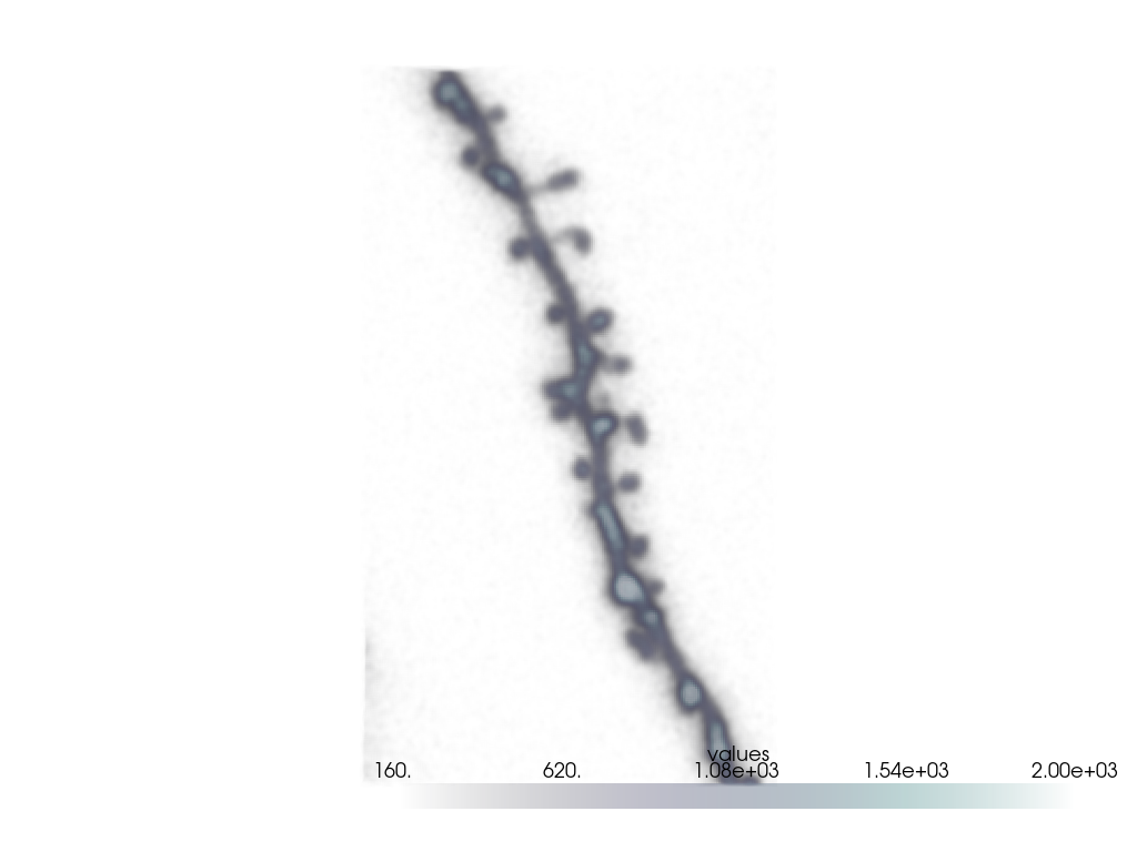
1. Load and Inspect the Data

We begin by loading the TIFF data, then visualize the image stack through the z-axis.

img = skimage.io.imread("dendrite.tif")


def _update0(i):
    mpl_img.set_array(img[i])
    return (mpl_img,)


fig, ax = plt.subplots(figsize=(7, 3))
mpl_img = ax.imshow(img[0], cmap="Greys_r", vmin=160, vmax=2000)
ax.set(xlim=(0, img.shape[2]), ylim=(0, img.shape[1]))
animation = matplotlib.animation.FuncAnimation(fig, _update0, len(img), interval=100, blit=True)
plt.show()

Once Loop Reflect

Visualize in 3D

Since we are fitting a 3D spline, let’s visualize the image stack in 3D.

grid = pv.ImageData(dimensions=np.array(img.shape) + 1)
grid.origin = (0, 0, 0)
grid.spacing = (1, 1, 1)
grid.cell_data["values"] = img.flatten(order="F")
plotter = pv.Plotter()
plotter.add_volume(grid, cmap="bone", clim=(160, 2000))
plotter.camera_position = "yz"
plotter.show()

Static Scene

Interactive Scene

NOTE: if you don’t see the image after switching to ‘Interactive Scene’ you might have to click and drag on the white space once.

2. Segmentation and Skeletonization

We segment the dendrite using Otsu’s method and skeletonize it to obtain the pixel coordinates for spline fitting.

thresh = skimage.filters.threshold_otsu(img)
mask = img > thresh
# Keep only the largest connected component
label_img = skimage.measure.label(mask)
label_biggest = np.argmax(np.bincount(label_img.flatten())[1:]) + 1
mask = label_img == label_biggest

# Skeletonize
skeleton = skimage.morphology.skeletonize(mask)

# Get skeleton coordinates
skeleton_points = np.stack(np.where(skeleton), axis=-1)

# Visualize skeleton
skeleton_point_cloud = pv.PolyData(skeleton_points.astype(float))
plotter = pv.Plotter()
plotter.add_volume(grid, cmap="bone", clim=(160, 2000))
plotter.add_mesh(skeleton_point_cloud, color=splinebox_color, point_size=10, render_points_as_spheres=True)
plotter.camera_position = "yz"
plotter.show()

Static Scene

Interactive Scene

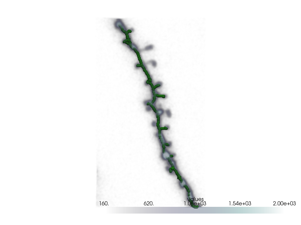
Extract the Longest Path of the Skeleton

We convert the skeleton into a graph and extract the longest path, which corresponds to the main dendrite.

# Returns a sparse connectivity matrix (graph) and the corresponding pixel coordinates
# for each knot in the graph.
graph, coords = skan.csr.skeleton_to_csgraph(skeleton)
coords = np.stack(coords, axis=-1)


# Use the shortest path algorithm to find the distances between all knots(skeleton points).
dist_matrix, predecessors = scipy.sparse.csgraph.shortest_path(graph, return_predecessors=True)

# Extract the index of the start and end knots of the longest path
start_index, stop_index = np.unravel_index(np.argmax(dist_matrix), dist_matrix.shape)

# Reconstruct the longest path using the predecessor matrix
i = start_index
skeleton_points = []
while i != stop_index:
    skeleton_points.append(coords[i])
    i = predecessors[stop_index, i]
skeleton_points = np.array(skeleton_points)

# Visualize longest path
skeleton_point_cloud = pv.PolyData(skeleton_points.astype(float))
plotter = pv.Plotter()
plotter.add_volume(grid, cmap="bone", clim=(160, 2000))
plotter.add_mesh(skeleton_point_cloud, color=splinebox_color, point_size=10, render_points_as_spheres=True)
plotter.camera_position = "yz"
plotter.show()

Static Scene

Interactive Scene

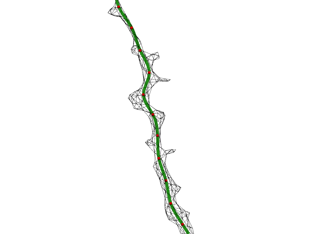
3. Fit a Spline

Now that we have the main points of the dendrite, we fit a spline.

M = 20
basis_function = splinebox.basis_functions.B3()
spline = splinebox.spline_curves.Spline(M=M, basis_function=basis_function, closed=False)
spline.fit(skeleton_points)

4. Plot the Fitted Spline

Let’s visualize the spline and its knots along with the segmented dendrite.

# Creat meshes for the spline and the knots of the spline
t = np.linspace(0, M - 1, M * 15)
spline_mesh = pv.MultipleLines(points=spline(t))
knots_point_cloud = pv.PolyData(spline.knots)

# Prepare segmentation mesh
grid = pv.ImageData(dimensions=mask.shape)
mesh = grid.contour([0.5], mask.flatten(order="F"), method="marching_cubes")
mesh = mesh.clean()
mesh = mesh.decimate(0.98)
mesh = mesh.smooth(100)

plotter = pv.Plotter()
plotter.add_mesh(mesh, style="wireframe", color="black")
plotter.add_mesh(spline_mesh, color=splinebox_color, line_width=10)
plotter.add_mesh(knots_point_cloud, color="red", point_size=10, render_points_as_spheres=True)
plotter.camera_position = "yz"
plotter.zoom_camera(2)
plotter.show()

Static Scene

Interactive Scene

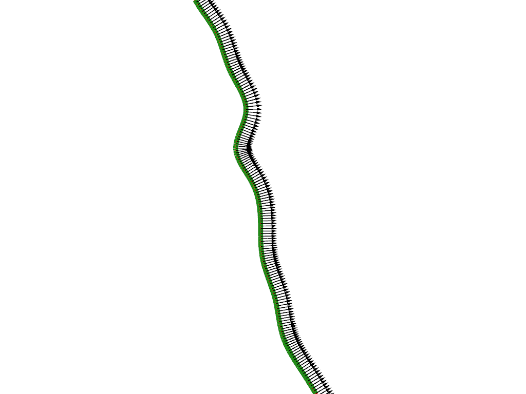
5. Compute Normal Planes

To align the image coordinate system with the spline, we compute normal planes along the spline. The normal planes are spanned by two vectors, which are normal to the local derivative vector of the spline (i.e. the vector pointing in the local direction of the spline).

# Compute derivative vectors along the spline
deriv = spline(t, derivative=1)

Compute the first normal vector

We select the normal vector that lies in the x-y plane (i.e. we set the z component to zero).

normal1 = np.zeros((len(t), 3))
normal1[:, 1] = deriv[:, 2]
normal1[:, 2] = -deriv[:, 1]

Compute the second normal vector

The second normal vector can be obtained using the cross product. This yields a vector that is perpendicular to the two input vectors deriv and normal1.

normal2 = np.zeros((len(t), 3))
normal2 = np.cross(deriv, normal1)

# Normalize vectors
normal1 /= np.linalg.norm(normal1, axis=1)[:, np.newaxis]
normal2 /= np.linalg.norm(normal2, axis=1)[:, np.newaxis]

Visualize Normal Planes

We scale the vectors for better visibility and plot them to verify they are perpendicular to the spline.

spline_mesh["normal1"] = normal1 * 7
spline_mesh["normal2"] = normal2 * 7

plotter = pv.Plotter()
spline_mesh.set_active_vectors("normal1")
plotter.add_mesh(spline_mesh.arrows, lighting=False, color="black")
spline_mesh.set_active_vectors("normal2")
plotter.add_mesh(spline_mesh.arrows, lighting=False, color="red")
plotter.add_mesh(spline_mesh, color=splinebox_color, line_width=10)
plotter.camera_position = "yz"
plotter.zoom_camera(2)
plotter.show()

Static Scene

Interactive Scene

Extract Pixel Values in Normal Planes

Finally, we interpolate pixel values from the original image along the computed normal planes.

# Centers of the normal planes
spline_coordinates = spline(t)

# Coefficients for scaling the normal vectors
half_window_size = 25
window_range = np.arange(-half_window_size, half_window_size)
ii, jj = np.meshgrid(window_range, window_range)

# Compute pixel coordinates using scaled normal vectors
normal_planes = np.multiply.outer(ii, normal1) + np.multiply.outer(jj, normal2)

# Fix the order of the axes (spline position first, before the normal directions)
normal_planes = np.rollaxis(normal_planes, 2, 0)

# Position normal planes on spline
normal_planes += spline_coordinates[:, np.newaxis, np.newaxis]

# Interpolate pixel values
shape = normal_planes.shape
vals = scipy.ndimage.map_coordinates(
    img,
    normal_planes.reshape(-1, 3).T,
    order=1,
)
vals = vals.reshape(shape[:-1]).astype(np.float64)

# Mask out pixels outside the volume
mask = (
    (np.min(normal_planes, axis=3) < 0)
    | (normal_planes[:, :, :, 0] > img.shape[0] - 1)
    | (normal_planes[:, :, :, 1] > img.shape[1] - 1)
    | (normal_planes[:, :, :, 2] > img.shape[2] - 1)
)
vals[mask] = np.nan

6. Animate the Dendrite-Centric Image

We create an animation showing the dendrite as seen along the fitted spline.

def _update1(i):
    mpl_point.set_offsets(
        spline_coordinates[
            i,
            2:0:-1,
        ].T
    )
    mpl_img.set_array(vals[i])
    return (mpl_point, mpl_img)


fig, axes = plt.subplots(1, 2, figsize=(7, 3))
axes[0].imshow(np.max(img, axis=0), cmap="Greys_r", vmin=160, vmax=2000)
mpl_point = axes[0].scatter((spline_coordinates[0, 2],), (spline_coordinates[0, 1],))
mpl_img = axes[1].imshow(vals[0], cmap="Greys_r", vmin=160, vmax=2000)
axes[1].set(xlim=(0, vals.shape[2]), ylim=(0, vals.shape[1]))
axes[1].scatter((half_window_size,), (half_window_size,))
animation = matplotlib.animation.FuncAnimation(fig, _update1, len(vals), interval=100, blit=True)
plt.show()

Once Loop Reflect