Performance Comparison: splinebox vs scipy

In this example, we will compare the performance of splinebox against scipy in three tasks:

1. Spline creation

2. Spline evaluation

3. Data fitting

We will measure the time required for each task across different numbers of knots, spline dimensionalities, and whether the spline is open or closed.

import time

import matplotlib.pyplot as plt
import numpy as np
import pandas as pd
import scipy
import seaborn as sns
import splinebox

# Number of times each task is repeated for more reliable results
n_repetitions = 10
# Number of knots
Ms = np.arange(10, 101, 10)

Spline Creation and Evaluation

First, we compare the time taken to create splines and evaluate them. We repeat the measurements 11 times, discarding the first due to numba’s Just-In-Time (JIT) compilation overhead, which is cached for future runs.

results_creation = []
results_evaluation = []

# Evaluate both open and closed splines
for closed in [True, False]:
    # Dimensionalities: 1D, 2D, 3D, 10D
    for ndim in (1, 2, 3, 10):
        for M in Ms:
            for repetition in range(n_repetitions + 1):
                knots = np.random.rand(M, ndim)

                # Measure splinebox creation time
                start = time.perf_counter_ns()
                spline = splinebox.Spline(M, splinebox.B3(), closed=closed)
                spline.knots = knots
                stop = time.perf_counter_ns()

                if repetition != 0:
                    results_creation.append(
                        [
                            "splinebox",
                            f"{ndim}D",
                            M,
                            "closed" if closed else "open",
                            stop - start,
                        ]
                    )

                # Measure spline evaluation time for different number of parameter values (nt)
                for nt in [10, 100, 1000, 10000]:
                    t = np.linspace(0, M if closed else M - 1, nt)
                    start_eval = time.perf_counter_ns()
                    spline(t)
                    stop_eval = time.perf_counter_ns()

                    if repetition != 0:
                        results_evaluation.append(
                            [
                                "splinebox",
                                f"{ndim}D",
                                M,
                                nt,
                                "closed" if closed else "open",
                                stop - start,
                            ]
                        )

                # Measure scipy spline creation time
                if closed:
                    start = time.perf_counter_ns()
                    t_knots = np.arange(M + 1)
                    knots_periodic = np.concatenate([knots, knots[0][np.newaxis, :]], axis=0)
                    spline = scipy.interpolate.make_interp_spline(t_knots, knots_periodic, k=3, bc_type="periodic")
                    stop = time.perf_counter_ns()
                else:
                    start = time.perf_counter_ns()
                    t_knots = np.arange(M)
                    spline = scipy.interpolate.make_interp_spline(t_knots, knots, k=3, bc_type="natural")
                    stop = time.perf_counter_ns()

                if repetition != 0:
                    results_creation.append(
                        [
                            "scipy",
                            f"{ndim}D",
                            M,
                            "closed" if closed else "open",
                            stop - start,
                        ]
                    )

                # Measure scipy spline evaluation time
                for nt in [10, 100, 1000, 10000]:
                    t = np.linspace(0, M if closed else M - 1, nt)
                    start_eval = time.perf_counter_ns()
                    spline(t)
                    stop_eval = time.perf_counter_ns()
                    if repetition != 0:
                        results_evaluation.append(
                            [
                                "scipy",
                                f"{ndim}D",
                                M,
                                nt,
                                "closed" if closed else "open",
                                stop - start,
                            ]
                        )

Plotting Spline Creation Time

Now, that we have collected all of the times, we can turn the results into a data frame and plot the results using seaborn.

# Convert results to DataFrame and plot the creation times
df = pd.DataFrame(results_creation, columns=["Package", "Dimensionality", "Number of knots", "closed", "time [ns]"])
for periodicity in ["closed", "open"]:
    fig, ax = plt.subplots()
    ax.set(yscale="log")
    sns.set_palette(sns.color_palette(["#228b18", "#0053a6"]))
    sns.lineplot(
        x="Number of knots",
        y="time [ns]",
        hue="Package",
        style="Dimensionality",
        data=df.loc[df["closed"] == periodicity],
        ax=ax,
    )
    plt.title(f"Creation of {periodicity} splines")
    plt.show()

• 
• 

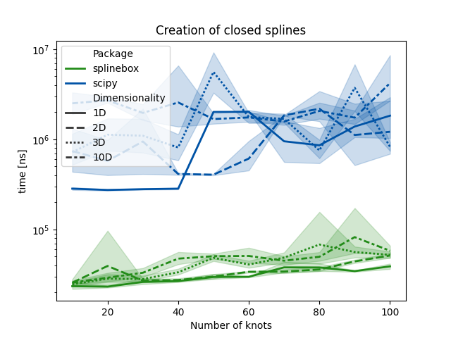
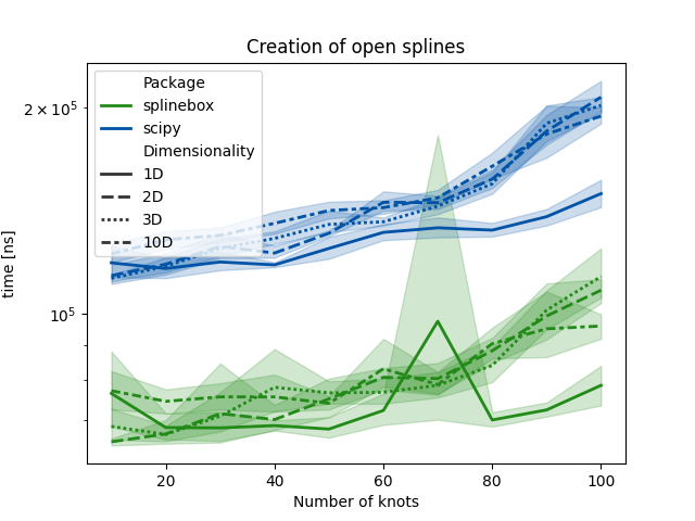
The results show that splinbox outperforms scipy in all condition for the task of creating a spline from a given set of knots.

Plotting Spline Evaluation Time

# Convert evaluation results to DataFrame and plot
df = pd.DataFrame(
    results_evaluation,
    columns=["Package", "Dimensionality", "Number of knots", "Number of parameter values", "closed", "time [ns]"],
)
for periodicity in ["closed", "open"]:
    fig, ax = plt.subplots(figsize=(7, 7))
    ax.set(yscale="log")
    sns.set_palette(sns.color_palette(["#228b18", "#0053a6"]))
    sns.lineplot(
        x="Number of knots",
        y="time [ns]",
        hue="Package",
        style="Number of parameter values",
        data=df.loc[df["closed"] == periodicity],
        ax=ax,
    )
    plt.title(f"Evaluation of {periodicity} splines")
    plt.show()

• 
• 

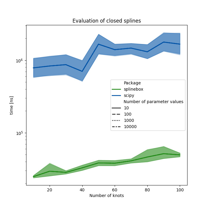
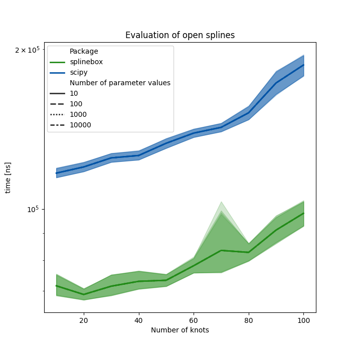
Once again, splinebox outperforms scipy, in all conditions for the spline evaluation task.

Data Fitting

Now, we compare the time it takes for splinebox and scipy to fit data, i.e., determine control points for a spline with M knots using least-squares fitting.

results_fitting = []

for closed in [True, False]:
    for ndim in (1, 2, 3, 10):
        for M in Ms:
            for repetition in range(n_repetitions + 1):
                data = np.random.rand(M * 10, ndim)

                # Measure splinebox fitting time
                start = time.perf_counter_ns()
                spline = splinebox.Spline(M, splinebox.B3(), closed=closed)
                spline.fit(data)
                stop = time.perf_counter_ns()

                if repetition != 0:
                    results_fitting.append(
                        [
                            "splinebox",
                            f"{ndim}D",
                            M,
                            "closed" if closed else "open",
                            stop - start,
                        ]
                    )

                # Measure scipy fitting time
                k = 3
                if closed:
                    start = time.perf_counter_ns()
                    N = len(data)
                    t = np.arange(-k, M + k + 1)
                    u = np.linspace(0, M, N + 1)[:-1]
                    tck, u = scipy.interpolate.splprep(data.T, k=k, u=u, t=t, task=-1, s=0, per=N)
                    stop = time.perf_counter_ns()

                else:
                    start = time.perf_counter_ns()
                    N = len(data)
                    t = np.arange(-k, M + k)
                    u = np.linspace(0, M - 1, N)
                    tck, u = scipy.interpolate.splprep(data.T, k=k, u=u, t=t, task=-1, s=0)
                    stop = time.perf_counter_ns()

                if repetition != 0:
                    results_fitting.append(
                        [
                            "scipy",
                            f"{ndim}D",
                            M,
                            "closed" if closed else "open",
                            stop - start,
                        ]
                    )

Plotting Fitting Time

df = pd.DataFrame(
    results_fitting,
    columns=["Package", "Dimensionality", "Number of knots", "closed", "time [ns]"],
)
for periodicity in ["closed", "open"]:
    fig, ax = plt.subplots(figsize=(7, 7))
    ax.set(yscale="log")
    sns.set_palette(sns.color_palette(["#228b18", "#0053a6"]))
    sns.lineplot(
        x="Number of knots",
        y="time [ns]",
        hue="Package",
        style="Dimensionality",
        data=df.loc[df["closed"] == periodicity],
        ax=ax,
    )
    plt.title(f"Fitting of {periodicity} splines")
    plt.show()

• 
• 

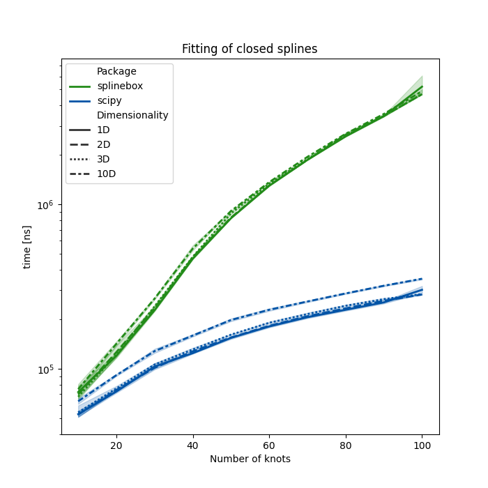
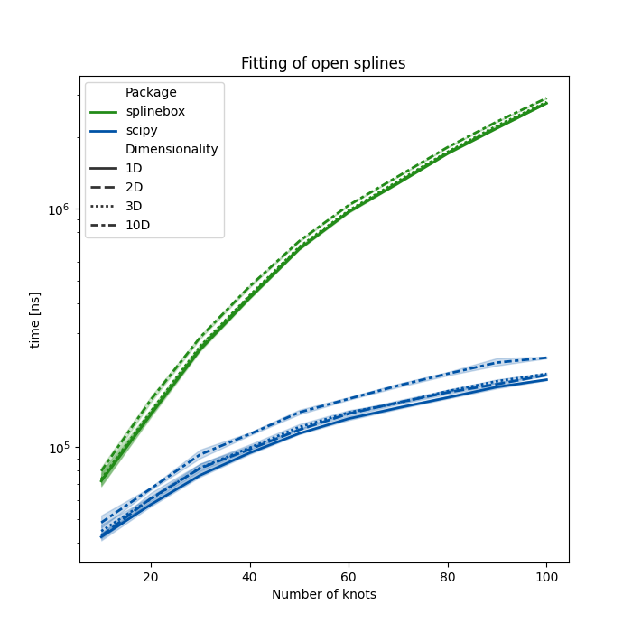
In the fitting task splinebox is outperformed by scipy’s splprep, but is competetive for splines with relatively few knots (i.e. < 20).

Results Summary

1. Spline Creation: splinebox consistently outperforms scipy across all dimensions for both open and closed splines.

2. Spline Evaluation: Similarly, splinebox is faster in evaluating splines, especially as the number of parameter values increases.

3. Data Fitting: While scipy has an edge in fitting tasks, particularly for splines with more than 20 knots, splinebox remains competitive for smaller splines.